Find the shadow edge in an image

In this notebook a demonstration is given how to find the shadow edge from an initial estimate. It uses a morphsnake, that either grows or shrinks towards a boundary.

import of funcitons from libraries

First we need to import some generic libraries for plotting and file management

import matplotlib.pyplot as plt

import os
import numpy as np
import morphsnakes as ms

Than more specific functions can be imported from the dhdt library

from dhdt.generic.mapping_io import read_geo_image
from dhdt.generic.handler_sentinel2 import get_s2_image_locations, get_s2_dict
from dhdt.generic.gis_tools import get_mask_boundary

from dhdt.input.read_sentinel2 import list_central_wavelength_msi, read_stack_s2, s2_dn2toa, read_mean_sun_angles_s2

from dhdt.preprocessing.shadow_transforms import apply_shadow_transform
from dhdt.preprocessing.shadow_filters import enhance_shadows
from dhdt.preprocessing.image_transforms import mat_to_gray, inverse_tangent_transformation

from dhdt.postprocessing.solar_tools import make_shading, make_shadowing

data preparation

Here some local data is taken, please adjust this to your own liking. A link to a Sentinel-2 directory is given, as well as, a link to a CopDEM elevation model of the same resolution.

dat_dir = '/Users/Alten005/surfdrive/Eratosthenes/RedGlacier/Sentinel-2/S2A_MSIL1C_20201019T213531_N0209_R086_T05VMG_20201019T220042.SAFE'

Z_file = "COP-DEM-05VMG.tif"
Z_dir = os.path.join('/Users/Alten005/surfdrive/Eratosthenes/RedGlacier/',
                      'Cop-DEM_GLO-30')

Z = read_geo_image(os.path.join(Z_dir, Z_file))[0]

A selection of bands is used here (only the 10m), and a random subset of the image is taken, so the details can be seen. Furthermore, most meta-data is extracted and put in a dataframe and a dictionary.

boi = ['red', 'green', 'blue', 'nir']
h,w = 100, 500
s2_df = list_central_wavelength_msi()
s2_df = s2_df[s2_df['common_name'].isin(boi)]
s2_df, datastrip_id = get_s2_image_locations(os.path.join(dat_dir, 'MTD_MSIL1C.xml'), s2_df)
s2_dict = get_s2_dict(s2_df)

Now the data can be loaded and cut to the subset.

im_stack, spatialRef, geoTransform, targetprj = read_stack_s2(s2_df)
im_stack = mat_to_gray(im_stack)
m,n = im_stack.shape[0], im_stack.shape[1]

j_min, i_min = np.random.randint(w, n-w), np.random.randint(h, m-h)
j_max, i_max = j_min + w, i_min + h

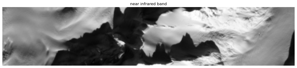
For convenience, the data can be plotted. Here the near infrared band is shown.

plt.rcParams['figure.figsize'] = [16.,4.]
plt.title('near infrared band'),
plt.imshow(inverse_tangent_transformation(4*im_stack[i_min:i_max,j_min:j_max,-1]), cmap=plt.cm.gray), plt.axis('off');

im_stack = im_stack[i_min:i_max,j_min:j_max,:]

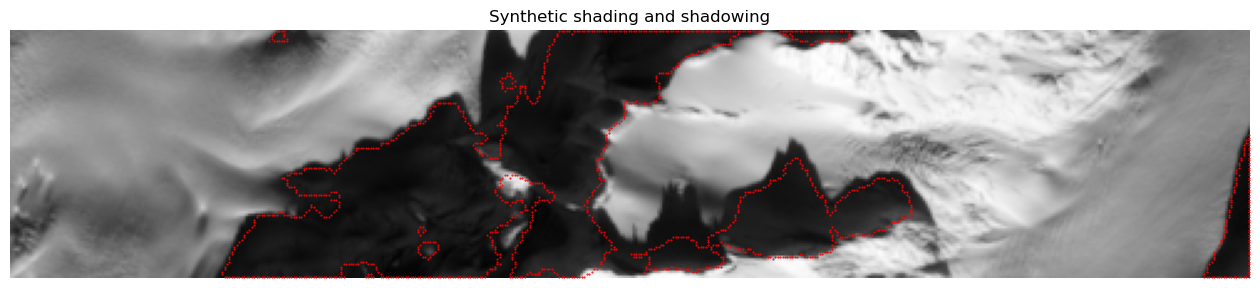
Since an elevation model is also loaded, a synthetic image can also be created. Which will hopefully ease the interpretation of the different methodologies later on.

sun_zn, sun_az = read_mean_sun_angles_s2(s2_dict['MTD_TL_path'])
Shw =  make_shadowing(Z.data, sun_az, sun_zn)
Shd =  make_shading(Z.data, sun_az, sun_zn)
Shw, Shd = Shw[i_min:i_max,j_min:j_max], Shd[i_min:i_max,j_min:j_max]

A visualization of a shading and a shadowing can now be created

S_bnd = get_mask_boundary(Shw)
iB,jB = np.where(S_bnd)

plt.rcParams['figure.figsize'] = [16.,4.]
plt.title('Synthetic shading and shadowing'),
plt.imshow(inverse_tangent_transformation(4*im_stack[i_min:i_max,j_min:j_max,-1]), cmap=plt.cm.gray)
plt.scatter(jB,iB,1,'red','.'), plt.axis('off');

i_bl = np.flatnonzero(s2_df['common_name']=='blue')[0]
i_gr = np.flatnonzero(s2_df['common_name'] == 'green')[0]
i_rd = np.flatnonzero(s2_df['common_name']=='red')[0]
i_nr = np.flatnonzero(s2_df['common_name'] == 'nir')[0]
S,R = apply_shadow_transform('entropy',im_stack[...,i_bl], im_stack[...,i_gr],im_stack[...,i_rd],[],
                             im_stack[...,i_nr], [], a=138.)

counts = 50 # iterations
M = ms.morphological_chan_vese(S, counts, init_level_set=Shw, albedo=R,
                               smoothing=1, lambda1=1, lambda2=1)

M_bnd = get_mask_boundary(M)
iM,jM = np.where(M_bnd)

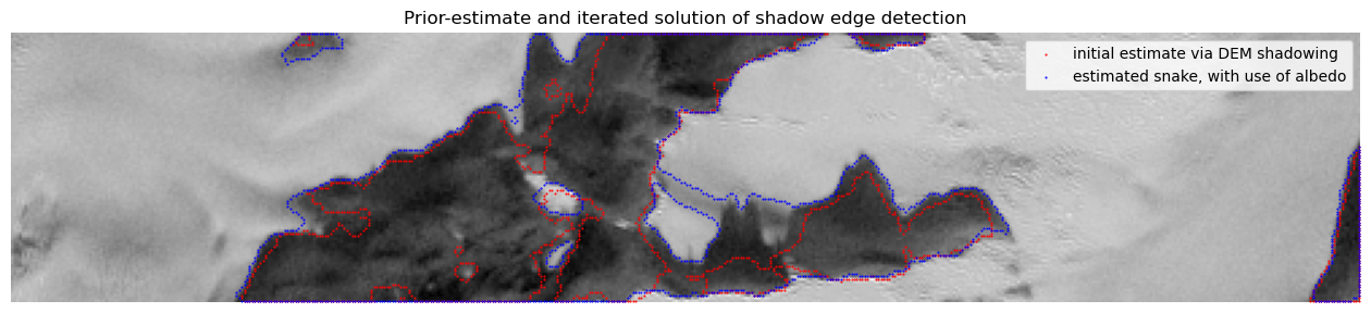
plt.rcParams['figure.figsize'] = [16.,4.]
plt.title('Prior-estimate and iterated solution of shadow edge detection'),
plt.imshow(inverse_tangent_transformation(S), cmap=plt.cm.gray)
plt.scatter(jB,iB,1,'red','.'), plt.scatter(jM,iM,1,'blue','.'), plt.axis('off');
plt.legend({'initial estimate via DEM shadowing','estimated snake, with use of albedo'});